Note

This tutorial is also available on nbviewer, offering an alternative platform for your learning convenience.

🔥 Free Pandas Course: https://hedaro.gumroad.com/l/tqqfq

Description:

Hey friend, imagine you’re a data analyst for a popular fashion retailer, and you need to analyze customer purchase behavior. The company wants to understand which products are frequently bought together, identify trends in customer purchases and preferences, and optimize marketing strategies accordingly.

Tasks:

Product Category Optimization: Merge two datasets (customer purchases and product categories) to identify which product categories have the highest average order value.
Product Analysis: Create a summary table to identify and display the top-selling product (ranked #1) for each month of every year.
Customer Purchase Trends: Transform the data to show the monthly purchase trends for each customer segment (e.g., age group, location). Use grouping and aggregation to calculate average monthly purchases.

# import libraries
import pandas as pd
import numpy as np
import sys
 
print('Python version ' + sys.version)
print('Pandas version ' + pd.__version__)
print('Numpy version ' + np.__version__)

Python version 3.11.7 | packaged by Anaconda, Inc. | (main, Dec 15 2023, 18:05:47) [MSC v.1916 64 bit (AMD64)]
Pandas version 2.2.1
Numpy version 1.26.4

The Data

This dataset represents a fashion retailer’s customer purchase behavior, consisting of approximately 5,000 purchases made by 1,000 customers across 50 products, with details on customer demographics, product information and purchase history. The data includes customer ID, age, location, product ID, product name, category, purchase date and order value.

Columns:

CustomerID: Unique customer identifier.
Age: Customer age.
Location: Customer location (Urban/Rural).
ProductID: Unique product identifier.
ProductName: Product name (18-64 years of age)
Category: Product category (Clothing/Accessories/Footwear).
PurchaseID: Unique purchase identifier.
PurchaseDate: Date of purchase.
OrderValue: Total value of the purchase.

# set the seed
np.random.seed(0)
 
# customer data
customer_data = pd.DataFrame({
    'CustomerID': np.arange(1, 1001),
    'Age': np.random.randint(18, 65, 1000),
    'Location': np.random.choice(['Urban', 'Rural'], 1000)
})
 
# product data
product_data = pd.DataFrame({
    'ProductID': np.arange(1, 51),
    'ProductName': [f'Product {i}' for i in range(1, 51)],
    'Category': np.random.choice(['Clothing', 'Accessories', 'Footwear'], 50)
})
 
# purchase data
purchase_data = pd.DataFrame({
    'PurchaseID': np.arange(1, 5001),
    'CustomerID': np.random.choice(customer_data['CustomerID'], 5000),
    'ProductID': np.random.choice(product_data['ProductID'], 5000),
    'PurchaseDate': pd.date_range('2022-01-01', periods=5000),
    'OrderValue': np.random.randint(10, 100, 5000)
})

Let us take a look at the data types for each dataframe.

customer_data.info()

<class 'pandas.core.frame.DataFrame'>
RangeIndex: 1000 entries, 0 to 999
Data columns (total 3 columns):
 #   Column      Non-Null Count  Dtype 
---  ------      --------------  ----- 
 0   CustomerID  1000 non-null   int32 
 1   Age         1000 non-null   int32 
 2   Location    1000 non-null   object
dtypes: int32(2), object(1)
memory usage: 15.8+ KB

product_data.info()

<class 'pandas.core.frame.DataFrame'>
RangeIndex: 50 entries, 0 to 49
Data columns (total 3 columns):
 #   Column       Non-Null Count  Dtype 
---  ------       --------------  ----- 
 0   ProductID    50 non-null     int32 
 1   ProductName  50 non-null     object
 2   Category     50 non-null     object
dtypes: int32(1), object(2)
memory usage: 1.1+ KB

purchase_data.info()

<class 'pandas.core.frame.DataFrame'>
RangeIndex: 5000 entries, 0 to 4999
Data columns (total 5 columns):
 #   Column        Non-Null Count  Dtype         
---  ------        --------------  -----         
 0   PurchaseID    5000 non-null   int32         
 1   CustomerID    5000 non-null   int32         
 2   ProductID     5000 non-null   int32         
 3   PurchaseDate  5000 non-null   datetime64[ns]
 4   OrderValue    5000 non-null   int32         
dtypes: datetime64[ns](1), int32(4)
memory usage: 117.3 KB

Product Category Optimization

Merge two datasets (customer purchases and product categories) to identify which product categories have the highest average order value. Use data reshaping to present the results.

Note: the .merge() method performs an inner join by default. This means only the rows where “ProductID” matches between the two dataframes will be returned.

# merge the product and purchase dataframes
df = purchase_data.merge(product_data, on='ProductID')
df.head()

	PurchaseID	CustomerID	ProductID	PurchaseDate	OrderValue	ProductName	Category
0	1	525	8	2022-01-01	25	Product 8	Accessories
1	2	430	10	2022-01-02	31	Product 10	Footwear
2	3	520	40	2022-01-03	53	Product 40	Clothing
3	4	507	46	2022-01-04	92	Product 46	Footwear
4	5	432	34	2022-01-05	20	Product 34	Footwear

# create group object
group = df.groupby('Category')
 
# get the average OrderValue of group
group['OrderValue'].mean().sort_values(ascending=False)

Category
Accessories    55.083221
Footwear       55.024229
Clothing       54.106714
Name: OrderValue, dtype: float64

Product Analysis

Create a summary table to identify and display the top-selling product (ranked #1) for each month of every year.

Note: The tricky piece to this task is that after we group by the month-year and count the number of products sold suring that time period, we need to select the top-selling product. Grouping and then counting that group is the easy part. Selecting n number of rows from that group is the part that is a little harder to do.

To convert a date object into YYYY-MONTH, use:

%Y - Extract the year
%B - Extract the full month name

df['PurchaseDate'][:5].dt.strftime('%Y-%B')

0    2022-January
1    2022-January
2    2022-January
3    2022-January
4    2022-January
Name: PurchaseDate, dtype: object

# create year_month column
df['year_month'] = df['PurchaseDate'].dt.strftime('%Y-%B')
df.head()

	PurchaseID	CustomerID	ProductID	PurchaseDate	OrderValue	ProductName	Category	year_month
0	1	525	8	2022-01-01	25	Product 8	Accessories	2022-January
1	2	430	10	2022-01-02	31	Product 10	Footwear	2022-January
2	3	520	40	2022-01-03	53	Product 40	Clothing	2022-January
3	4	507	46	2022-01-04	92	Product 46	Footwear	2022-January
4	5	432	34	2022-01-05	20	Product 34	Footwear	2022-January

The first step is to create a new dataset that has the frequency each “ProductName” shows up in a specific Year-Month combination. Remember these products represents sales made on that particular date.

Here is a summary of what we are doing in the code below:

Create a group object that includes the “year_month” and “ProductName” columns
We then count the number of times the product was sold on that “year_month” using count()
Since the dataframe has multiple columns, I just picked “PurchaseID”. The rest of the columns should all have the same values
.reset_index is used so the columns “year_month” and “ProductName” are moved from the index into a regular dataframe column
I then renamed the “PurchaseID” column to “count” as that is what it represents

We end up with a new dataset that tells us how many times a specific product was sold the month of every year.

# group by year-month and ProductName
group = df.groupby(['year_month', 'ProductName'])
 
# generate the ProductName frequency dataset
year_month_df = group.count()['PurchaseID'] \
                     .reset_index() \
                     .rename(columns={'PurchaseID': 'count'})
 
year_month_df.head()

	year_month	ProductName	count
0	2022-April	Product 1	1
1	2022-April	Product 10	1
2	2022-April	Product 11	1
3	2022-April	Product 13	3
4	2022-April	Product 22	2

Now we can grab the top-selling product on a particular date. We clean up the data a bit so that at the end we end up with the specific “id” that will point to the name of the Product we are after.

Let me explain what this “id” column represents:
The dataframe named “year_month_df” contains an index. Do you see it? Every row contains an index value and this index value is what we see in the dataframe named “n_largest”.

If we take the first row, we see a value of 3 under the “id” column. This value of 3 is pointing to the row in the “year_month_df” dataframe that has an index value of 3.

This means the row: 2022-April, Product 13, 3

We then will end up with a dataframe named “n_largest” that has all of the top-selling Products for a specific year-month combination. For those curious, you can update nlargest(1) to any other number to get for example the top 2 selling products.

n_largest = year_month_df.groupby('year_month')['count'] \
                         .nlargest(2) \
                         .reset_index()[['year_month','level_1']] \
                         .rename(columns={'level_1': 'id'})
n_largest.head()

	year_month	id
0	2022-April	3
1	2022-April	17
2	2022-August	33
3	2022-August	22
4	2022-December	57

We then use the `.merge()’ method to lookup the “ProductName” associated with the “id” column.

results = year_month_df.merge(n_largest, left_index=True, right_on='id')[['year_month_x','ProductName']]
results.head()

	year_month_x	ProductName
0	2022-April	Product 13
1	2022-April	Product 50
3	2022-August	Product 20
2	2022-August	Product 33
5	2022-December	Product 20

Another simpler approach might be to simply sort the data and use the .head(n) method.

def get_top_n(df, n):
    return df.sort_values(['year_month', 'count'], ascending=[True, False]) \
             .groupby('year_month').head(n).reset_index(drop=True)    
 
# group by year-month and ProductName
group = df.groupby(['year_month', 'ProductName'])
 
# generate the ProductName frequency dataset
year_month_df = group.count()['PurchaseID'] \
                     .reset_index() \
                     .rename(columns={'PurchaseID': 'count'}) \
                     .pipe(get_top_n, 1)
 
year_month_df.head()

	year_month	ProductName	count
0	2022-April	Product 13	3
1	2022-August	Product 33	3
2	2022-December	Product 39	3
3	2022-February	Product 20	2
4	2022-January	Product 27	3

Customer Purchase Trends

Transform the data to show the monthly purchase trends for each customer segment (e.g., age group, location). Use grouping and aggregation to calculate average monthly purchases.

# merge the customer, product and purchase dataframes
df = purchase_data.merge(product_data, on='ProductID') \
                  .merge(customer_data, on='CustomerID')
df.head()

	PurchaseID	CustomerID	ProductID	PurchaseDate	OrderValue	ProductName	Category	Age	Location
0	1	525	8	2022-01-01	25	Product 8	Accessories	24	Rural
1	2	430	10	2022-01-02	31	Product 10	Footwear	18	Urban
2	3	520	40	2022-01-03	53	Product 40	Clothing	50	Urban
3	4	507	46	2022-01-04	92	Product 46	Footwear	39	Rural
4	5	432	34	2022-01-05	20	Product 34	Footwear	54	Urban

# create year_month column
df['year_month'] = df['PurchaseDate'].dt.strftime('%Y-%m')
df.head()

	PurchaseID	CustomerID	ProductID	PurchaseDate	OrderValue	ProductName	Category	Age	Location	year_month
0	1	525	8	2022-01-01	25	Product 8	Accessories	24	Rural	2022-01
1	2	430	10	2022-01-02	31	Product 10	Footwear	18	Urban	2022-01
2	3	520	40	2022-01-03	53	Product 40	Clothing	50	Urban	2022-01
3	4	507	46	2022-01-04	92	Product 46	Footwear	39	Rural	2022-01
4	5	432	34	2022-01-05	20	Product 34	Footwear	54	Urban	2022-01

# create group object
object = df.groupby(['year_month','Location'])
 
# calculate average monthly purchases on the group
result = object['OrderValue'].mean()
result.head()

year_month  Location
2022-01     Rural       57.857143
            Urban       64.117647
2022-02     Rural       51.500000
            Urban       50.500000
2022-03     Rural       42.615385
Name: OrderValue, dtype: float64

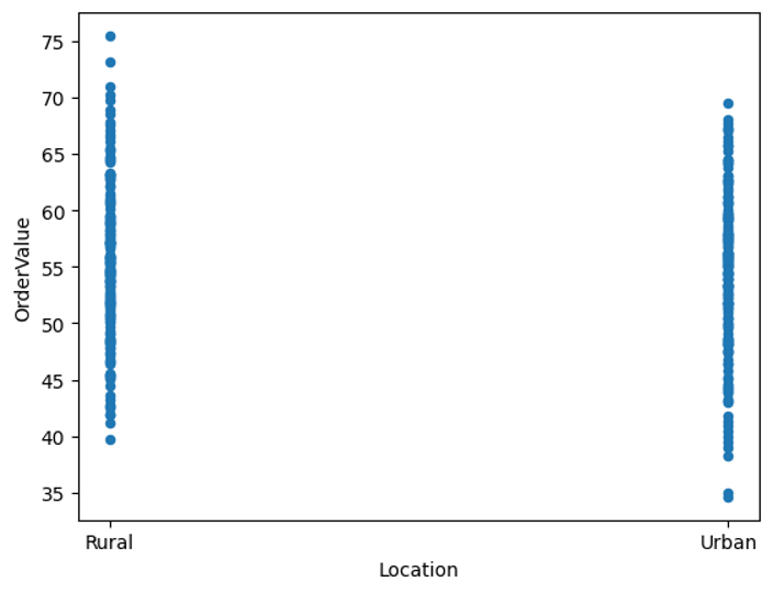
We can see that “Rural” customers seem to have higher orders than “Urban” customers.

result.reset_index().plot.scatter(x='Location',y='OrderValue');

# create group object
object = df.groupby(['year_month','Age'])
 
# calculate average monthly purchases on the group
result = object['OrderValue'].mean()
result.head()

year_month  Age
2022-01     18     64.333333
            20     73.000000
            21     80.000000
            22     85.000000
            24     25.000000
Name: OrderValue, dtype: float64

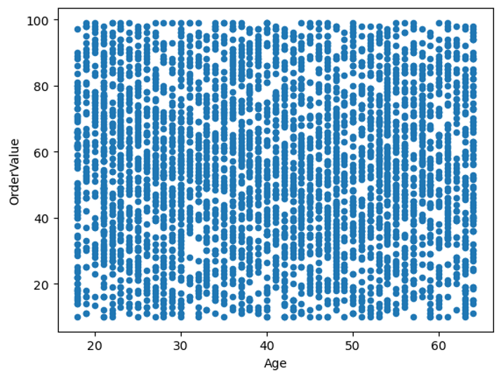
No patterns identified for the customers ages.

result.reset_index().plot.scatter(x='Age',y='OrderValue');

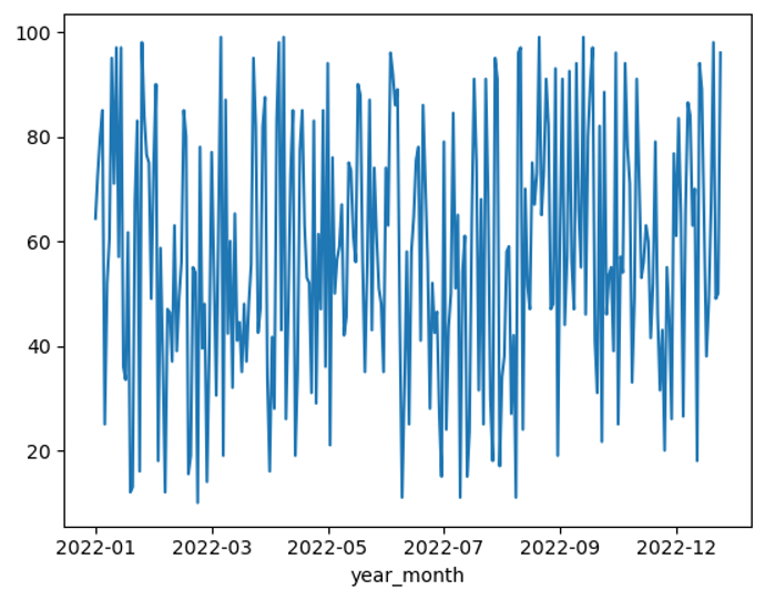
If we take a look at the year 2022 as a sample of the dataset, I am not able to see any trends in the data.

result.reset_index().set_index('year_month')[:'2022-12']['OrderValue'].plot();

Summary

You have gained hands-on experience analyzing customer purchase behavior for a fashion retailer using Pandas.

Key Skills Acquired

Merge datasets
Group and aggregate data
Visualize trends
Identify patterns in customer purchasing behavior

You can now apply these skills to real-world data analysis tasks, uncovering valuable insights in customer behavior and preferences.

Key Takeaways

Merging datasets using pd.merge().
Grouping and aggregating data using groupby() and mean().
Reshaping data using reset_index() and rename().
Filtering top-selling products using nlargest() or sort_values() and head().
Visualizing data using plot.scatter().

Hedaro

Explorer

Customer Purchase Analysis for a Fashion Retailer

Description:

Tasks:

The Data

Columns:

Product Category Optimization

Product Analysis

Customer Purchase Trends

Summary

Key Skills Acquired

Key Takeaways

Graph View

Table of Contents

Backlinks

Hedaro

Explorer

Customer Purchase Analysis for a Fashion Retailer

Description: §

Tasks: §

The Data §

Columns: §

Product Category Optimization §

Product Analysis §

Customer Purchase Trends §

Summary §

Key Skills Acquired §

Key Takeaways §

Graph View

Table of Contents

Backlinks

Description:

Tasks:

The Data

Columns:

Product Category Optimization

Product Analysis

Customer Purchase Trends

Summary

Key Skills Acquired

Key Takeaways