Note
- This tutorial is also available on nbviewer, offering an alternative platform for your learning convenience.
- 🔥 Free Pandas Course: https://hedaro.gumroad.com/l/tqqfq
Description:
Imagine you’re the Data Scientist for a professional soccer league. The season is heating up, and the league wants to gain insights into team and player performance. They’ve collected a vast dataset of match statistics, but it’s a bit of a mess. That’s where you come in!
Tasks:
- Goal Scoring Analysis: Calculate the top 5 teams with the highest median goal scoring per match, and display the results in a bar chart.
- Player Performance: Create a histogram showing the distribution of assists among all players in the season.
- Matchup Insights: Determine the teams with the highest winning percentage when playing at home, and display the results in a sorted table.
# import libraries
import pandas as pd
import numpy as np
import sys

print('Python version ' + sys.version)
print('Pandas version ' + pd.__version__)
print('Numpy version ' + np.__version__)
Python version 3.11.7 | packaged by Anaconda, Inc. | (main, Dec 15 2023, 18:05:47) [MSC v.1916 64 bit (AMD64)]
Pandas version 2.2.1
Numpy version 1.26.4
The Data
This dataset contains 500 matches, with team and player performance statistics. Your task is to wrangle this data using pandas to extract valuable insights!
Columns:
- match_id: a unique identifier for each match.
- team_home and team_away: IDs of the teams playing in each match, ranging from 0 to 19. These IDs don’t correspond to specific team names, but rather represent different teams in the simulation.
- goals_home and goals_away: the number of goals scored by each team in each match.
- player_assists and player_goals: the number of assists and goals scored by a player in each match.
Good luck, and have fun!
# set the seed
np.random.seed(0)

# declare variables
matches = 500
teams = 20
players = 500

data = {
    'match_id': np.arange(matches),
    'team_home': np.random.choice(teams, matches),
    'team_away': np.random.choice(teams, matches),
    'goals_home': np.random.poisson(lam=1.5, size=matches),
    'goals_away': np.random.poisson(lam=1.0, size=matches)
}

# create dataframe
df = pd.DataFrame(data)

# ensure player does not score more than the team
df['player_goals'] = df.apply(lambda x: np.minimum(np.random.poisson(lam=0.2, size=1), np.maximum(np.random.choice([x['goals_home'], x['goals_away']], 1), 0))[0], axis=1)

# ensure player does have more assists than goals scored
df['player_assists'] = df.apply(lambda x: np.minimum(np.random.poisson(lam=0.2, size=1), np.maximum(np.random.choice([x['player_goals']], 1), 0))[0], axis=1)

df.head()| match_id | team_home | team_away | goals_home | goals_away | player_goals | player_assists | |
|---|---|---|---|---|---|---|---|
| 0 | 0 | 12 | 0 | 2 | 0 | 0 | 0 |
| 1 | 1 | 15 | 9 | 0 | 0 | 0 | 0 |
| 2 | 2 | 0 | 16 | 3 | 2 | 1 | 0 |
| 3 | 3 | 3 | 2 | 0 | 2 | 0 | 0 |
| 4 | 4 | 3 | 8 | 2 | 1 | 0 | 0 |
We are expecting all of the columns to be numeric, let’s take a look and verify this.
df.info()<class 'pandas.core.frame.DataFrame'>
RangeIndex: 500 entries, 0 to 499
Data columns (total 7 columns):
# Column Non-Null Count Dtype
--- ------ -------------- -----
0 match_id 500 non-null int32
1 team_home 500 non-null int32
2 team_away 500 non-null int32
3 goals_home 500 non-null int32
4 goals_away 500 non-null int32
5 player_goals 500 non-null int32
6 player_assists 500 non-null int32
dtypes: int32(7)
memory usage: 13.8 KB
Goal Scoring Analysis:
Calculate the top 5 teams with the highest goal scoring average per match, and display the results in a bar chart.
home = df[['team_home','goals_home']]
home| team_home | goals_home | |
|---|---|---|
| 0 | 12 | 2 |
| 1 | 15 | 0 |
| 2 | 0 | 3 |
| 3 | 3 | 0 |
| 4 | 3 | 2 |
| … | … | … |
| 495 | 18 | 0 |
| 496 | 14 | 2 |
| 497 | 18 | 0 |
| 498 | 1 | 0 |
| 499 | 12 | 1 |
| 500 rows × 2 columns |
Note: We will try to use the median as the data is not Normally distributed.
You can see that for most of the away matches, the teams seem to score a median of 1 goal. For games where they have a home field advantage, we have a few teams scoring a median of 2 goals per game.
# home team
group = df.groupby('team_home')
group_home = group['goals_home'].median()

# away team
group = df.groupby('team_away')
group_away = group['goals_away'].median()

# combine data
combined = pd.concat([group_home, group_away], axis=1)

combined.plot.bar();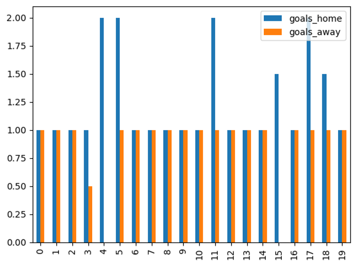
Let’s pull out top 5 scoring teams based on the median goals scored at home games. There was a tie for 5th place, team 18 and team 15 both scored a median of 1.5 goals per home game.
group_home.sort_values(ascending=False).head()team_home
11 2.0
17 2.0
4 2.0
5 2.0
18 1.5
Name: goals_home, dtype: float64
Player Performance:
Create a histogram showing the distribution of assists among all players in the season.
As you can see, most players do not have many assists according to the data
df['player_assists'].sort_values().hist();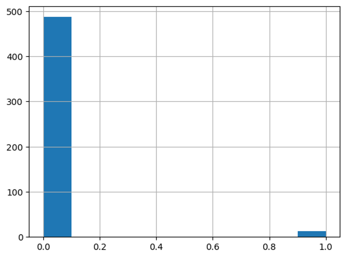
If we take a look at some descriptive statistics, we can conclude that there were very few high scoring/assisting players in the season.
df[['goals_home','goals_away','player_goals','player_assists']].describe()| goals_home | goals_away | player_goals | player_assists | |
|---|---|---|---|---|
| count | 500.000000 | 500.000000 | 500.000000 | 500.000000 |
| mean | 1.492000 | 1.040000 | 0.134000 | 0.026000 |
| std | 1.221852 | 0.990132 | 0.352552 | 0.159295 |
| min | 0.000000 | 0.000000 | 0.000000 | 0.000000 |
| 25% | 1.000000 | 0.000000 | 0.000000 | 0.000000 |
| 50% | 1.000000 | 1.000000 | 0.000000 | 0.000000 |
| 75% | 2.000000 | 2.000000 | 0.000000 | 0.000000 |
| max | 6.000000 | 5.000000 | 2.000000 | 1.000000 |
Conclusion
In this tutorial, we analyzed a dataset of soccer match statistics to gain insights into team and player performance. We calculated the top 5 teams with the highest median goal scoring per match and created a histogram showing the distribution of assists among all players.
What You Learned:
- How to calculate goal scoring averages per match
- How to visualize data using bar charts and histograms
- How to extract insights from data
Can you solve the BONUS question?
Matchup Insights: Determine the teams with the highest winning percentage when playing at home, and display the results in a sorted table.