Note
- This tutorial is also available on nbviewer, offering an alternative platform for your learning convenience.
- 🔥 Free Pandas Course: https://hedaro.gumroad.com/l/tqqfq
Some nifty ninjastics you can do with Group By and MatPlotLib.
import pandas as pd
from matplotlib.pylab import plt
import sys
Here is the csv data if you want to follow along:
Date,Symbol,Volume
1/1/2013,A,0
1/2/2013,A,200
1/3/2013,A,1200
1/4/2013,A,1001
1/5/2013,A,1300
1/6/2013,A,1350
3/8/2013,B,500
3/9/2013,B,1150
3/10/2013,B,1180
3/11/2013,B,2000
1/5/2013,C,56600
1/6/2013,C,45000
1/7/2013,C,200
5/20/2013,E,1300
5/21/2013,E,1700
5/22/2013,E,900
5/23/2013,E,2100
5/24/2013,E,8000
5/25/2013,E,12000
5/26/2013,E,1900
5/27/2013,E,1000
5/28/2013,E,1900
print('Python version ' + sys.version)
print('Pandas version ' + pd.__version__)
Python version 3.11.7 | packaged by Anaconda, Inc. | (main, Dec 15 2023, 18:05:47) [MSC v.1916 64 bit (AMD64)]
Pandas version 2.2.1
# let's see what kind of data we are working with
raw = pd.read_csv('Test_9_17_Python.csv')
raw.head()| Date | Symbol | Volume | |
|---|---|---|---|
| 0 | 1/1/2013 | A | 0 |
| 1 | 1/2/2013 | A | 200 |
| 2 | 1/3/2013 | A | 1200 |
| 3 | 1/4/2013 | A | 1001 |
| 4 | 1/5/2013 | A | 1300 |
df2 = raw.copy()You are going to have to change the data type of the Date column
df2.dtypesDate object
Symbol object
Volume int64
dtype: object
df2['Date'] = pd.to_datetime(df2['Date'])df2.dtypesDate datetime64[ns]
Symbol object
Volume int64
dtype: object
# generate some fake data
pool = ['boy','girl']
pool = pool*(int(len(df2)/2))
df2['Gender'] = pool
df = df2.copy()
df.head()| Date | Symbol | Volume | Gender | |
|---|---|---|---|---|
| 0 | 2013-01-01 | A | 0 | boy |
| 1 | 2013-01-02 | A | 200 | girl |
| 2 | 2013-01-03 | A | 1200 | boy |
| 3 | 2013-01-04 | A | 1001 | girl |
| 4 | 2013-01-05 | A | 1300 | boy |
Group one column and plot
group = df.groupby('Symbol')for x in group:
print(type(x))
print('//////')<class 'tuple'>
//////
<class 'tuple'>
//////
<class 'tuple'>
//////
<class 'tuple'>
//////
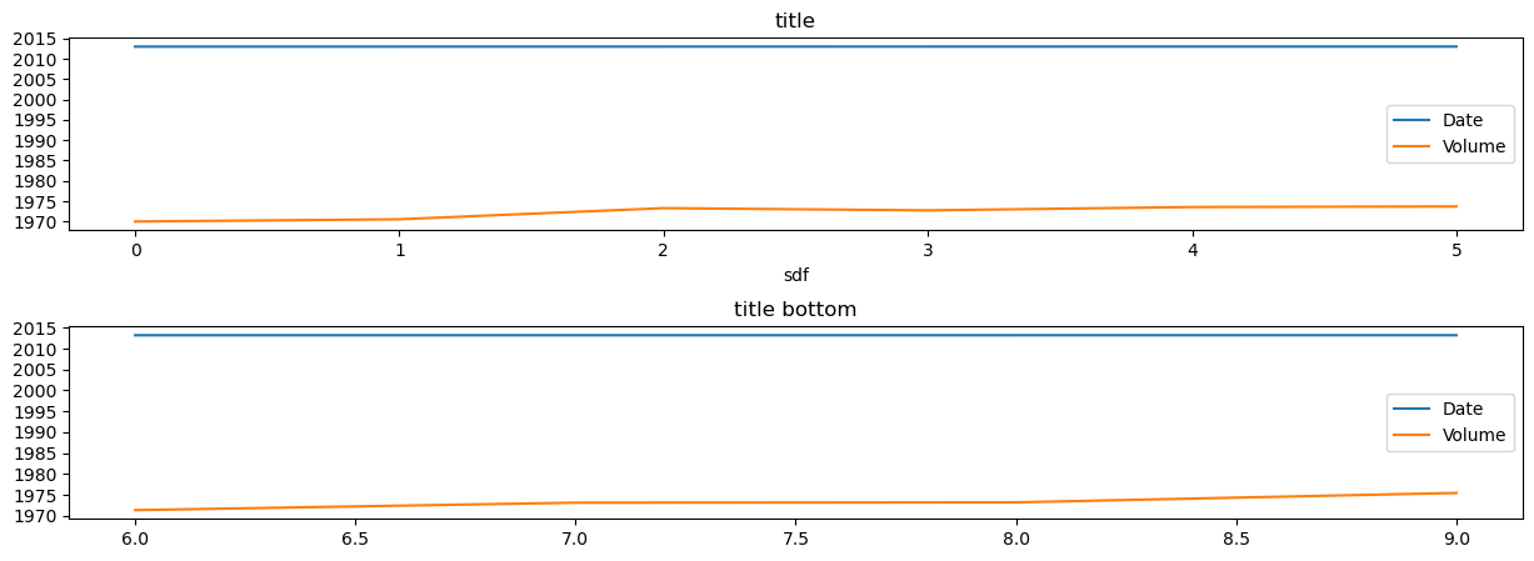
fig, axes = plt.subplots(2,1, figsize=(15,5))
plt.subplots_adjust(hspace=0.5)

group.get_group('A').plot(ax=axes[0])
group.get_group('B').plot(ax=axes[1])

axes[0].set_title('title')
axes[0].set_xlabel('sdf')

axes[1].set_title('title bottom');
def plot(group):
    mask = group['Volume'].apply(lambda x: x>1000)
    mask2 = group['Symbol'] == 'A'
    mask3 = group['Symbol'] == 'B'

    return group[mask & (mask2 | mask3)]['Volume'].sum()

a = group[['Symbol','Volume']].apply(plot)
a = pd.DataFrame(a)
a = a.rename(columns={0:'Volume'})
a.plot();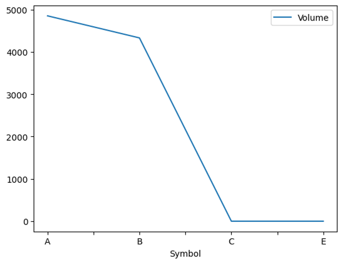
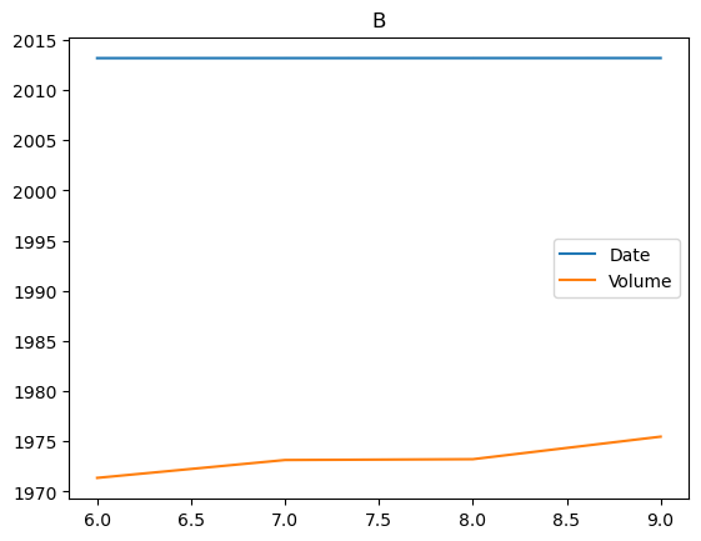
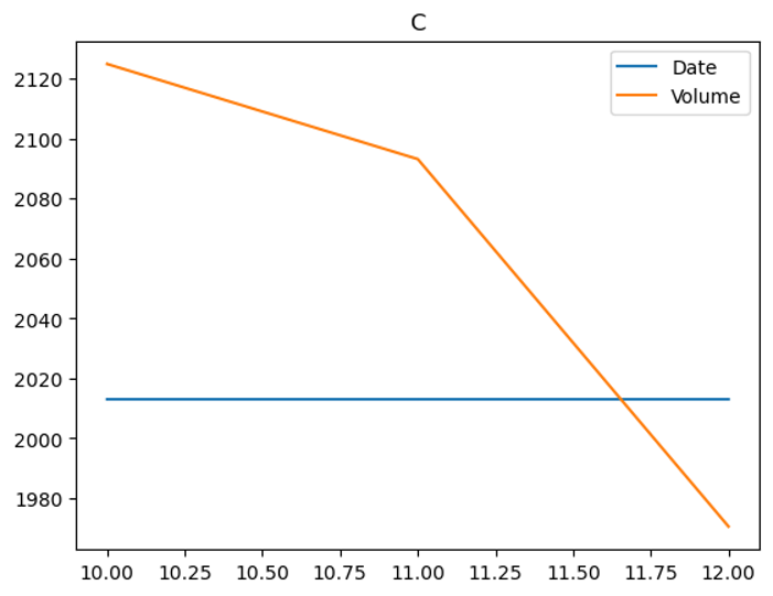
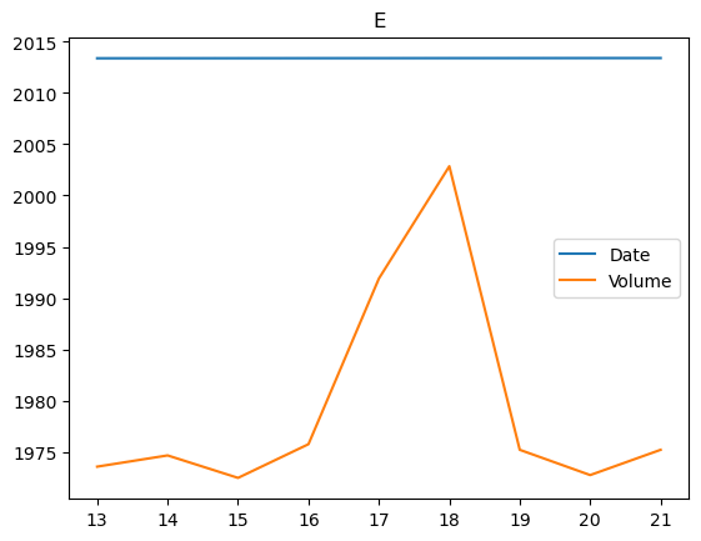
for i, g in group:
    g.plot(title=i)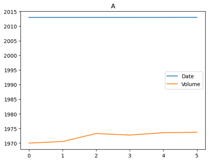
Group two columns and plot
group = df.groupby(['Symbol', 'Gender'])for i, g in group:
print(i)('A', 'boy')
('A', 'girl')
('B', 'boy')
('B', 'girl')
('C', 'boy')
('C', 'girl')
('E', 'boy')
('E', 'girl')
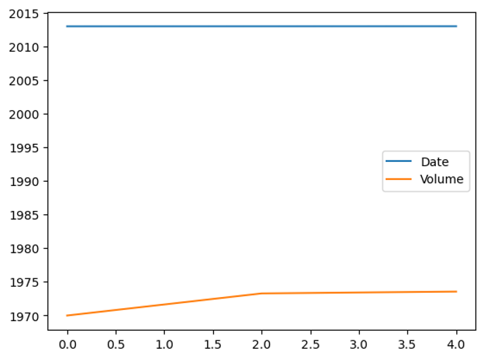
group.get_group(('A', 'boy')).plot()
group.get_group(('A', 'boy')).plot();
fig, axes = plt.subplots(len(group.groups),1, figsize=(5,20))
fig.subplots_adjust(hspace=1.0) ## Create space between plots
ix = 0

for i, g in group:
    p = g.plot(ax=axes[ix], title=str(i))
    if ix < len(axes)-1:
        ix = ix + 1
    else:
        ix = 0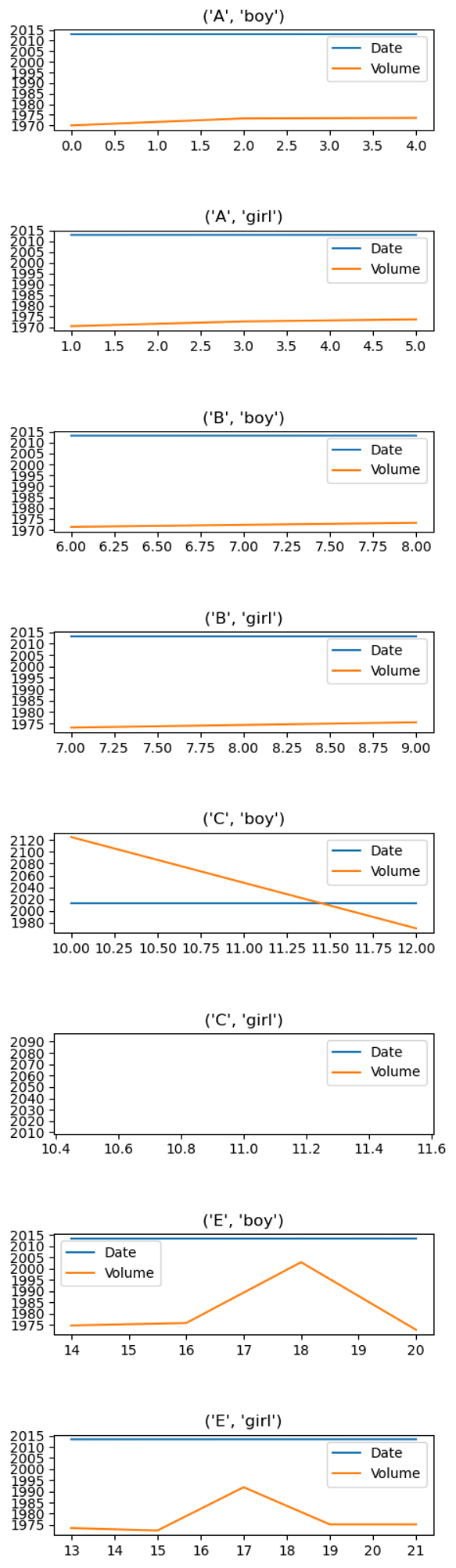
PANDAS HOME PAGE