Note
- This tutorial is also available on nbviewer, offering an alternative platform for your learning convenience.
- 🔥 Free Pandas Course: https://hedaro.gumroad.com/l/tqqfq
Description
You are a Fintech professional at a leading investment firm, and your team is responsible for generating quarterly reports for a client who invests in real estate. The client has a large portfolio of properties across the United States and needs to identify areas with the highest return on investment. Your task is to analyze a dataset of property sales and identify trends, patterns, and insights that will inform investment decisions.
Tasks
- Data Wrangling: Using the ‘Date’ column, extract the quarter and year of the sale. Create a new column ‘Sale Quarter’ in the format ‘Q1 2020’.
- Data Analysis: Calculate the total sales, average sale price, and return on investment (ROI) for each region and property type. ROI is calculated as (Sale Price - Purchase Price) / Purchase Price.
- Data Visualization: Create a dashboard to visualize the top-performing regions and property types, and identify areas with the highest growth potential.
# import libraries
import pandas as pd
import numpy as np
import matplotlib.pyplot as plt # only needed for advanced plotting
import matplotlib as mpl # only needed to get version
import sys

print('Python version ' + sys.version)
print('Pandas version ' + pd.__version__)
print('Numpy version ' + np.__version__)
print('matplotlib version: ' + mpl.__version__)
Python version 3.11.7 | packaged by Anaconda, Inc. | (main, Dec 15 2023, 18:05:47) [MSC v.1916 64 bit (AMD64)]
Pandas version 2.2.1
Numpy version 1.26.4
matplotlib version: 3.8.4
The Data
The dataset contains real estate sales data, comprising 10,000 records of property sales across the United States. The data provides insights into the real estate market, allowing for analysis of sales trends, investment opportunities, and regional performance.
Columns:
- Region: The region where the property is located (Northeast, Southwest, West, Southeast)
- Property Type: The type of property (Residential, Commercial, Industrial)
- Sale Price: The sale price of the property
- Purchase Price: The purchase price of the property
- Date: The date the property was sold
- Location: The location of the property (Urban, Rural, Suburban)
# set the seed
np.random.seed(0)

data = {
    'Region': np.random.choice(['Northeast', 'Southwest', 'West', 'Southeast'], size=10000),
    'Property Type': np.random.choice(['Residential', 'Commercial', 'Industrial'], size=10000),
    'Sale Price': np.random.randint(100000, 1000000, size=10000),
    'Purchase Price': np.random.randint(80000, 900000, size=10000),
    'Date': pd.date_range('2020-01-01', periods=10000, freq='D'),
    'Location': np.random.choice(['Urban', 'Rural', 'Suburban'], size=10000)
}

df = pd.DataFrame(data)
df.head()| Region | Property Type | Sale Price | Purchase Price | Date | Location | |
|---|---|---|---|---|---|---|
| 0 | Northeast | Commercial | 218584 | 773265 | 2020-01-01 | Rural |
| 1 | Southeast | Industrial | 178913 | 131066 | 2020-01-02 | Suburban |
| 2 | Southwest | Residential | 736016 | 736997 | 2020-01-03 | Suburban |
| 3 | Northeast | Industrial | 408411 | 603822 | 2020-01-04 | Suburban |
| 4 | Southeast | Industrial | 531722 | 280768 | 2020-01-05 | Rural |
Let us take a look at the data types. The code to generate the data was pretty basic, so I am not expecting any issues with the data types for this tutorial.
df.info()<class 'pandas.core.frame.DataFrame'>
RangeIndex: 10000 entries, 0 to 9999
Data columns (total 6 columns):
# Column Non-Null Count Dtype
--- ------ -------------- -----
0 Region 10000 non-null object
1 Property Type 10000 non-null object
2 Sale Price 10000 non-null int32
3 Purchase Price 10000 non-null int32
4 Date 10000 non-null datetime64[ns]
5 Location 10000 non-null object
dtypes: datetime64[ns](1), int32(2), object(3)
memory usage: 390.8+ KB
Data Wrangling:
Using the ‘Date’ column, extract the quarter and year of the sale. Create a new column ‘Sale Quarter’ in the format ‘Q1 2020’.
We can extract the day, the year, the month, and yes even the quarter from a date object.
.dt.year: extracts the year
.dt.month: extracts the month
.dt.day: extracts the day
.dt.hour: extracts the hour
.dt.minute: extracts the minute
.dt.second: extracts the second
.dt.microsecond: extracts the microsecond
.dt.quarter: extracts the quarter (Q1, Q2, Q3, or Q4)
.dt.dayofweek: extracts the day of the week (Monday=0, ..., Sunday=6)
.dt.dayofyear: extracts the day of the year the year
.dt.weekofyear: extracts the week of the year
.dt.days_in_month: The number of days in the month of the datetime
# let us verify quarter works
df['Date'].dt.quarter.unique()array([1, 2, 3, 4])
Method #1: Make sure to convert numerical columns into strings
df['Sale Quarter'] = "Q" + df['Date'].dt.quarter.astype('str') + " " + df['Date'].dt.year.astype('str')

df.head()| Region | Property Type | Sale Price | Purchase Price | Date | Location | Sale Quarter | |
|---|---|---|---|---|---|---|---|
| 0 | Northeast | Commercial | 218584 | 773265 | 2020-01-01 | Rural | Q1 2020 |
| 1 | Southeast | Industrial | 178913 | 131066 | 2020-01-02 | Suburban | Q1 2020 |
| 2 | Southwest | Residential | 736016 | 736997 | 2020-01-03 | Suburban | Q1 2020 |
| 3 | Northeast | Industrial | 408411 | 603822 | 2020-01-04 | Suburban | Q1 2020 |
| 4 | Southeast | Industrial | 531722 | 280768 | 2020-01-05 | Rural | Q1 2020 |
Method #2: When using apply, do not use .dt to access the dates.
df['Sale Quarter'] = df['Date'].apply(lambda x: "Q{} {}".format(x.quarter, x.year))

df.head()| Region | Property Type | Sale Price | Purchase Price | Date | Location | Sale Quarter | |
|---|---|---|---|---|---|---|---|
| 0 | Northeast | Commercial | 218584 | 773265 | 2020-01-01 | Rural | Q1 2020 |
| 1 | Southeast | Industrial | 178913 | 131066 | 2020-01-02 | Suburban | Q1 2020 |
| 2 | Southwest | Residential | 736016 | 736997 | 2020-01-03 | Suburban | Q1 2020 |
| 3 | Northeast | Industrial | 408411 | 603822 | 2020-01-04 | Suburban | Q1 2020 |
| 4 | Southeast | Industrial | 531722 | 280768 | 2020-01-05 | Rural | Q1 2020 |
Data Analysis:
Calculate the total sales, average sale price, and return on investment (ROI) for each region and property type.
ROI is calculated as (Sale Price - Purchase Price) / Purchase Price.
We need to first calculate the ROI and add it to our dataframe.
df['ROI'] = (df["Sale Price"] - df["Purchase Price"]) / df["Purchase Price"]

df.head()| Region | Property Type | Sale Price | Purchase Price | Date | Location | Sale Quarter | ROI | |
|---|---|---|---|---|---|---|---|---|
| 0 | Northeast | Commercial | 218584 | 773265 | 2020-01-01 | Rural | Q1 2020 | -0.717323 |
| 1 | Southeast | Industrial | 178913 | 131066 | 2020-01-02 | Suburban | Q1 2020 | 0.365060 |
| 2 | Southwest | Residential | 736016 | 736997 | 2020-01-03 | Suburban | Q1 2020 | -0.001331 |
| 3 | Northeast | Industrial | 408411 | 603822 | 2020-01-04 | Suburban | Q1 2020 | -0.323624 |
| 4 | Southeast | Industrial | 531722 | 280768 | 2020-01-05 | Rural | Q1 2020 | 0.893813 |
# create group object
group = df.groupby(['Region','Property Type'])

# total sales, average sale price, and return on investment (ROI) for each region and property type
stats = group.agg(
     total_sales=pd.NamedAgg(column="Sale Price", aggfunc="sum"),
     avg_sale_price=pd.NamedAgg(column="Sale Price", aggfunc="mean"),
     avg_roi=pd.NamedAgg(column="ROI", aggfunc="mean")
)

stats| total_sales | avg_sale_price | avg_roi | ||
|---|---|---|---|---|
| Region | Property Type | |||
| Northeast | Commercial | 478204953 | 543414.719318 | 0.569722 |
| Industrial | 441306378 | 545496.140915 | 0.613538 | |
| Residential | 445531386 | 544659.396088 | 0.542753 | |
| Southeast | Commercial | 438267095 | 552669.728878 | 0.585154 |
| Industrial | 484245809 | 547170.405650 | 0.702109 | |
| Residential | 467827932 | 553642.523077 | 0.693283 | |
| Southwest | Commercial | 487230479 | 567867.691142 | 0.720646 |
| Industrial | 468987824 | 552400.263840 | 0.602655 | |
| Residential | 468436616 | 547879.083041 | 0.626235 | |
| West | Commercial | 426445537 | 551675.985770 | 0.631625 |
| Industrial | 444369230 | 528381.961950 | 0.493232 | |
| Residential | 418329316 | 526863.118388 | 0.569282 |
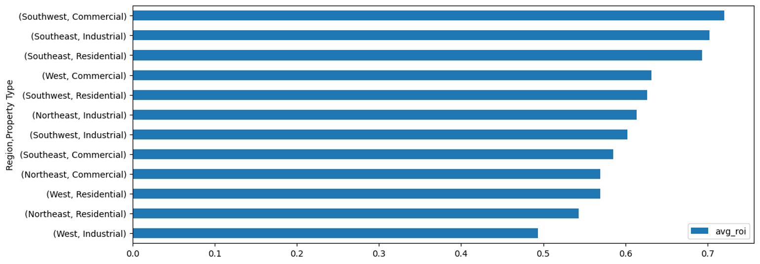
Data Visualization:
Create a dashboard to visualize the top-performing regions and property types, and identify areas with the highest growth potential.
Looking at the dashboard below, here are some key findings:
- Southeast (industrial and residential) and Southwest commercial have the best ROI
- Northeast commercial is the most expensive real estate sold but it has a very low ROI
Take note of all the MatPlotLib code I used to customize the plot, see how you can make use of it on your next visualization.
fig, axes = plt.subplots(nrows=1, ncols=2, figsize=(13, 5))
fig.subplots_adjust(hspace=0.25) ## Create space between plots

# Chart 1
stats[['avg_roi']].sort_values(by='avg_roi').plot.barh(figsize=(13, 5))

# Chart 2
stats[['total_sales']].sort_values(by='total_sales').head(3).plot.bar(ax=axes[0], legend=False)

# Chart 3
stats[['avg_sale_price']].sort_values(by='avg_sale_price').head(3).plot.bar(ax=axes[1], legend=False)

## customize viz ##

# Move the x-axis to the top of the plot
axes[0].spines['bottom'].set_position(('axes', 0.5))
axes[1].spines['bottom'].set_position(('axes', 0.5))

# hide ticks
axes[0].tick_params(axis='x', which='both', length=0)
axes[1].tick_params(axis='x', which='both', length=0)
axes[0].spines['bottom'].set_visible(False)
axes[1].spines['bottom'].set_visible(False)

# hide labels
axes[0].set_xlabel('')
axes[1].set_xlabel('')

# Rotate the x-axis labels 90 degrees and change text to white
axes[0].tick_params(axis='x', rotation=90, labelcolor='white')
axes[1].tick_params(axis='x', rotation=90, labelcolor='white')

# set titles to top two charts
axes[0].set_title('Total Sales')
axes[1].set_title('Average Sale Price');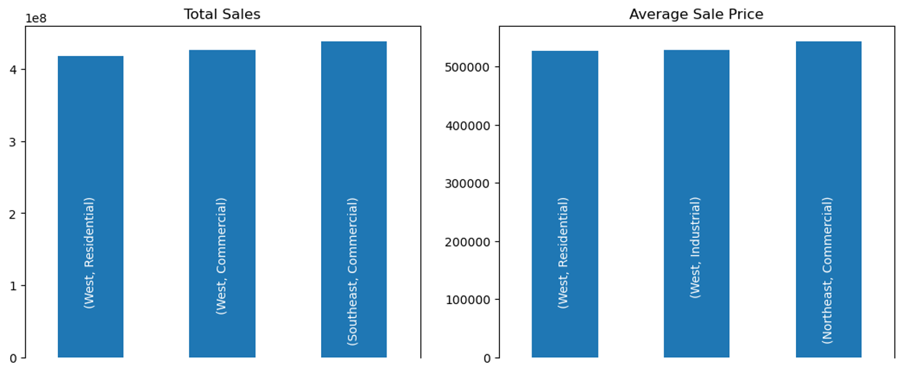
Summary:
The tutorial demonstrates how to extract insights from a real estate sales dataset using Pandas. It starts by creating a sample dataset and then performs data wrangling, analysis, and visualization to identify top-performing regions and property types.
Key Takeaways:
- Extracted the quarter and year from the ‘Date’ column and created a new ‘Sale Quarter’ column.
- Converted numerical columns to strings for proper formatting.
- Calculated the return on investment (ROI) for each property.
- Grouped data by region and property type to calculate total sales, average sale price, and average ROI.
- Created a dashboard with three charts to visualize top-performing regions and property types.
- Customized the plots using MatPlotLib to enhance visualization.